DBS101_Unit6

UNIT 6: Database Systems: Indexing, Query Processing, and Optimization

Introduction

In this blog post, I’ll share my understanding of three critical components that make databases efficient and powerful: indexing mechanisms, query processing techniques, and optimization strategies. These concepts form the backbone of any robust database management system, enabling rapid data retrieval and efficient query execution even when dealing with massive datasets.

What Are Indexes?

Indexes are special lookup tables (or data structures in document databases) that the database search engine uses to speed up data retrieval. They function much like the index at the back of a book, allowing the database to quickly locate the data without scanning every row in a table.

Without indexes, every query would require reading the entire contents of every relation it uses. This would be prohibitively expensive for queries that only fetch a few records, such as retrieving a single student record or records corresponding to a specific student in a “takes” relation.

Types of Indices

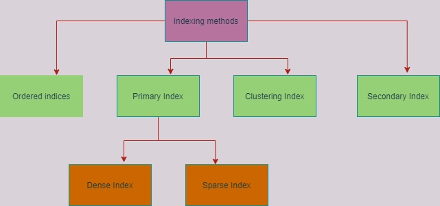
There are two primary types of indices:

1. Ordered Indices: Store values in a sorted order and associate each search key with records containing it.
2. Hashed Indices: Distribute values uniformly across buckets using a hash function.

Ordered Indices: Clustering vs. Non-Clustering

Based on how records are organized within files, ordered indices can be categorized as:

• Clustering Index (Primary Index): Records in the file are stored in the same sorted order as the index entries. Each index entry contains a search key value and a pointer to the first record with that key.

• Non-clustering Index (Secondary Index): Records in the file are not sorted in the same order as the index entries. Each index entry contains a search key value and pointers to all records with that key.

Dense vs. Sparse Indices

Ordered indices can be further classified based on their entry density:

• Dense Index: An index entry exists for every search-key value in the file. In a dense clustering index, each entry points to the first record with that search-key value. In a dense non-clustering index, each entry stores pointers to all records with the same search-key value.

• Sparse Index: An index entry exists for only some of the search-key values. Sparse indices can only be used if the relation is stored in sorted order of the search key (i.e., it’s a clustering index).

Multilevel Indexing

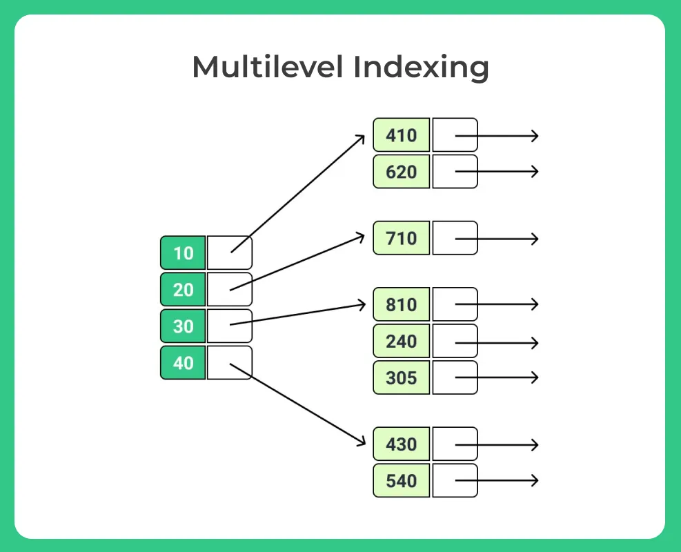
When indexing large relations, the index itself may not fit entirely in memory, which increases search time due to multiple disk block reads. Multilevel indexing addresses this problem by creating an index on the index itself:

• The main index (inner index) is stored on disk.
• A smaller outer index containing a subset of entries from the inner index is created and can fit entirely in memory.

To search for a value:

1. Binary search is performed on the in-memory outer index to find the range where the value would exist in the inner index.
2. Only the relevant blocks of the inner index are read from disk and searched.

This approach significantly reduces disk I/O operations when searching large indices.

B-Tree Family

The B-tree family represents the most widely used index structures that maintain efficiency despite insertions and deletions of data.

B-Tree: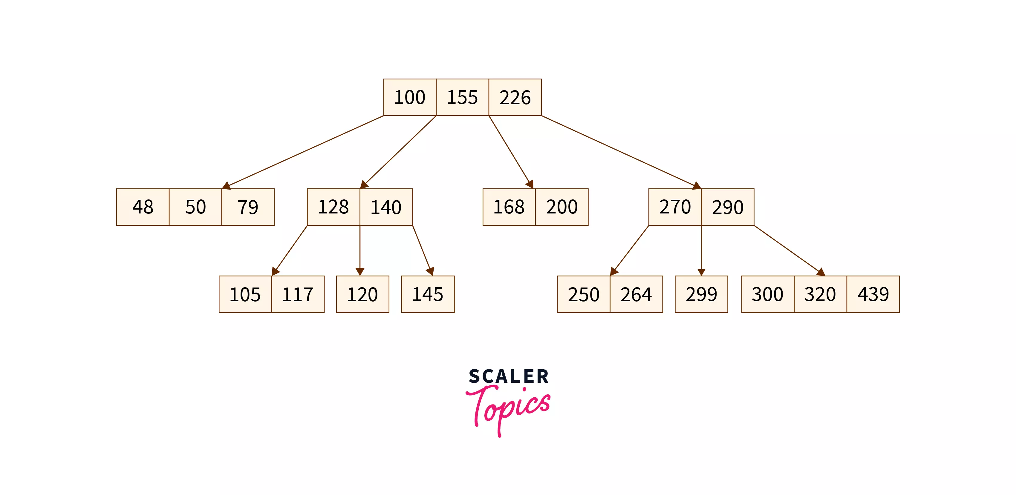

• A self-balancing search tree where each node can contain multiple keys and children.
• A generalized form of the binary search tree.
• Also known as a height-balanced m-way tree.

B+ Tree: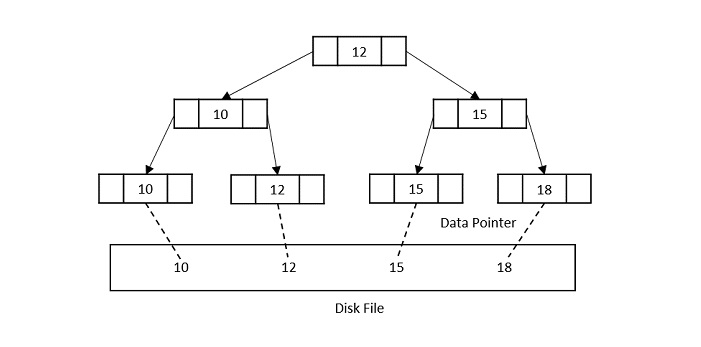

• The most commonly used index structure in databases.
• All data records are stored at the leaf level.
• Inner nodes only contain keys for guiding the search.
• Leaf nodes are linked, allowing for efficient range queries.

The B+ Tree offers several advantages:

• It’s perfectly balanced (every leaf node is at the same depth).
• Every node other than the root is at least half-full.
• Inner nodes with k keys have k+1 non-null children.
• Supports efficient search, insertion, and deletion operations.

Query Processing: From SQL to Results

What is Query Processing?

Query processing refers to the range of activities involved in extracting data from a database. These activities include:

1. Translating queries from high-level languages (like SQL) into expressions that can be used at the physical level.
2. Optimizing queries through various transformations.
3. Evaluating queries to produce results.

Steps in Query Processing

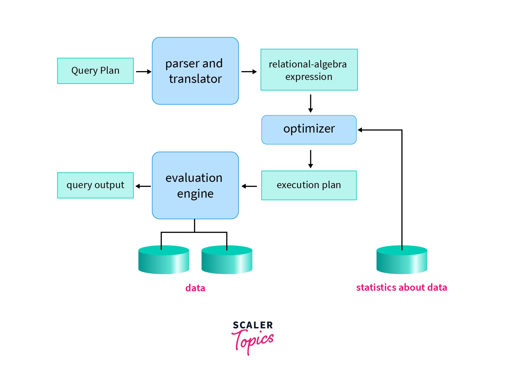
The query processing pipeline consists of three main steps:

1. Parsing and Translation:
   • Syntax checking and validation of relations.
   • Parsing into a parse tree.
   • Translation into a relational algebra expression.
   • Handling views by substituting their definitions.
2. Optimization:
   • Finding the most efficient query plan.
   • Choosing algorithms and access methods.
   • Determining join order and operation scheduling.
3. Evaluation:
   • Executing the query plan.
   • Retrieving and processing data.
   • Producing the final result.

Query Evaluation

SQL is a declarative language that doesn’t specify how to execute a query. To evaluate an SQL query, the database system:

1. Converts it to relational algebra (which is procedural).
2. Creates a query execution plan.
3. Executes the plan to produce results.

Measures of Query Cost

When evaluating the efficiency of query execution plans, several cost factors are considered:

1. Disk I/O Cost:
   • Number of blocks transferred (b).
   • Number of random I/O accesses (S).
   • Average block transfer time (tT).
   • Average block access time (tS) = disk seek time + rotational latency.

   The total cost can be calculated as: Cost = b * tT + S * tS.

2. CPU Cost:
   • While traditionally less significant than I/O cost, CPU cost becomes more important with modern storage technologies like SSDs and in-memory databases.

Query Execution

Query execution involves two main approaches:

1. Materialization:
   • Intermediate results are stored in temporary relations.
   • Each operation is executed completely before the next one starts.
   • Results are written to disk and read back when needed.
2. Pipelining:
   • Results are passed directly from one operation to the next.
   • Avoids creating and reading temporary relations.
   • Can start generating results early.
   • Implemented through iterators (open, next, close) or producer-consumer models.

Query Optimization: Making Queries Efficient

What is Query Optimization?

Query optimization is the process of selecting the most efficient query-evaluation plan from among the many strategies possible for processing a given query. This is especially important for complex queries where the difference between a good and bad execution plan can be orders of magnitude in performance.

Transformation of Relational Expressions

Relational algebra expressions can be transformed into equivalent expressions with different evaluation costs. Two expressions are equivalent if they generate the same set of tuples on every legal database instance.

Equivalence Rules

Some key equivalence rules include:

1. Conjunctive selection can be deconstructed: σθ1∧θ2(E) ≡ σθ1(σθ2(E)).
2. Selection operations are commutative: σθ1(σθ2(E)) ≡ σθ2(σθ1(E)).
3. Theta joins are commutative: E1 ⋈θ E2 ≡ E2 ⋈θ E1.
4. Natural joins are associative: (E1 ⋈ E2) ⋈ E3 ≡ E1 ⋈ (E2 ⋈ E3).
5. Selection distributes over join: σθ1(E1 ⋈θ E2) ≡ (σθ1(E1)) ⋈θ E2 (if θ1 only involves E1).

Join Ordering

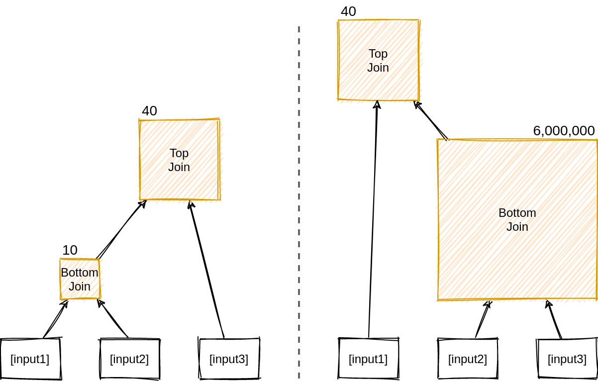
Join ordering is crucial for query optimization as it can dramatically affect the size of intermediate results. Consider this example:

The first join order (Customer WHERE region='Asia') JOIN Orders JOIN LineItems is more efficient because it filters customers early, creating a small intermediate relation.

The second order (Orders JOIN LineItems) JOIN (Customer WHERE region='Asia') produces a large intermediate relation by joining orders and line items first, only to discard most tuples in the second join.

Cost-Based Optimization

Cost-based optimization explores the space of all equivalent query evaluation plans:

1. Uses equivalence rules to generate alternative plans.
2. Estimates the cost of each plan based on statistics.
3. Chooses the plan with the lowest estimated cost.

This process covers two main aspects:

• Join order selection.
• Choosing join algorithms (nested loop, hash join, etc.).

Optimization Heuristics

To reduce the cost of optimization itself, database systems employ various heuristics:

• Perform selections early to reduce data size.
• Perform projections early after selections.
• Use left-deep join trees (easier for pipelining).
• Cache plans for repeated queries with different constants.

Practical Implementation Examples

Creating and Using Indices

Here’s how you can create different types of indices in PostgreSQL:

```sql – Create a dense index on employee ID CREATE INDEX employees_idx ON employees (emp_id);

– Create a dense non-clustering index on department CREATE INDEX employees_dept_idx ON employees (department);

– Create a sparse clustering index with one entry per block CREATE INDEX employees_sparse_idx ON employees (salary) WITH (fillfactor=100);